Due: 11:59pm March 9, 2021 (ET)

---

Overview

In this assignment you will implement simple linear regression and analyze multiple linear regression. Check out Seeing Theory for help understanding these concepts!

---

---

Assignment

You will modify util.py, simple_regression.py, and multiple_regression.py using bike_sharing.csv. You will be implementing most parts of the regressions from scratch. Here are some restrictions on the use of Python libraries for this assignment:

You cannot use sklearn.

For simple linear regression, you are allowed to use statsmodel and numpy only for calculating the MSE.

You can use statsmodel for multiple linear regression.

Pandas is only allowed for loading the dataset.

You will also submit written_questions.txt with your answers to the questions for Part 3.

---

Simple and Multiple Linear Regression

Linear Regression

Regression is used to predict numerical values given inputs. Linear regression attempts to model the line of best fit that explains the relationship between two or more variables by fitting a linear equation to observed data. One or more variables are considered to be the independent (or explanatory) variables, and one variable is considered to be a dependent (or response) variable. In simple linear regression, there is one independent variable and in multiple linear regression, there are two or more independent variables.

Before attempting to fit a linear model to observed data, a modeler should first determine whether or not there is a linear relationship between the variables of interest. This does not necessarily imply that one variable causes the other. Remember, correlation does not necessarily imply causation. For example, moderate alcohol consumption is correlated to longevity. This doesn’t necessarily mean that moderate alcohol consumption causes longevity. Another independent characteristic of moderate drinkers (extrovert lifestyle) might be responsible for longevity. Regardless, there is some association between the two variables. The goal in linear regression is to tease apart whether a correlation is likely to be a causal relationship, by controlling for these other variables/characteristics that might be confounding the analysis.

In simple linear regression, scatter plot can be a helpful tool in visually determining the strength of the relationship between two variables. The independent variable is typically plotted on the x-axis and the dependent variable is typically plotted on the y-axis. If there appears to be no association between the proposed explanatory and dependent variables (i.e., the scatter plot does not indicate any clear increasing or decreasing trends), then fitting a linear regression model to the data probably will likely not provide a useful model. (Note this is not always the case--just as confounding variables might lead a correlation to appear stronger than it is, it might also lead a relationship to appear weaker than it is.)

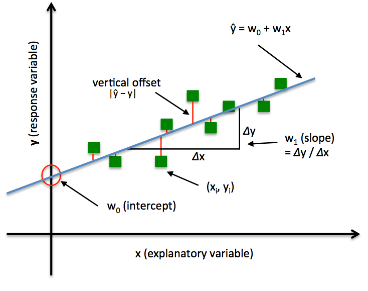
Shown in the picture below, in simple regression, we have a single feature x and weights w0 for the intercept and w1 for slope of the line. Our goal is to find the line that minimizes the vertical offsets, otherwise known as residuals. In other words, we define the best-fitting line as the line that minimizes the residual sum of squares (SSR or RSS) between our target variable y and our predicted output over all samples i in our training examples n.

A valuable numerical measure of association between two variables is the correlation coefficient , which is a value between -1 and 1 indicating the strength of the association of the observed data for the two variables. A simple linear regression line has an equation of the form Y = a + bX, where X is the independent (explanatory) variable and Y is the dependent variable. The slope of the line is b, and a is the intercept (the value of y when x = 0). A multiple linear regression line has an equation of the form Y = a + b_1X_1 + b_2 X_2 + … + b_n X_n for n independent variables.

Another useful metric is the R-squared value. This tells us how much of the variation in Y can be explained by the variation in X. The value for R-squared ranges from 0 to 1, and the closer to 1, the greater proportion of the variability in Y is explained by the variability in X. For more explanation on R-squared and how to calculate it, read here (this will be very helpful in Part 2!)

Do not confuse correlation and regression. Correlation is a numerical value that quantifies the degree to which two variables are related. Regression is a type of predictive analysis that uses a best fit line (Y = a + bX) that predicts Y given the value of X).

Part I: Data Preprocessing (18 Points)

Data & Functions Overview

Inside the data folder, bike_sharing.csv contains data of a two-year historical log corresponding to years 2011 and 2012 from Capital Bikeshare system, Washington D.C., USA. There are 11 different independent variables that you are attempting to predict and one dependent variable (the Count of Use of Bike). More information on the dataset can be found in README_data.txt.

The data functions described below are in util.pyand can be used for both simple and multilple linear regressions.

Load Data

In util.py, first implement load_data, which should load the data into X, and y variables using pandas. Make sure to load the correct dependent and independent variables when implementing and calling this function.

Train/Test Split

Then, fill in the functions split_data_randomly and train_test_split to randomly split the data into train and test datasets. You should create the following variables:X_train, X_test, y_train, y_test. A common convention in data science is to make 80% of the data the training data and 20% the test data. In train_test_split, we have provided test_pct = 0.2; use this in your split_data_randomly function to obtain this 80/20 split. You will train your model on the training data and test it on the test data.

Note that we expect you to distribute the data randomly, look into how you can use Python random.random to do this. In simple_regression.py and multiple_regression.py, we set random.seed(1) to guarrantee that we obtain the same split on every run. Please do not change this.

Lastly, when splitting data make sure that X,y pairs remain intact, that is, every X and its corresponding Y should both be in the same list(either test or train) and at the same index to make sure your model is accurate. To do this, we recommend using Python zip to form pairs before splitting the data into train and test sets.

Note: calculate_r_squared function is for the next section, and you don't need to implement it at this stage.

Part II: Simple Linear Regression (22 points)

The management team of Capital Bikeshare system wants to know how much weather conditions can predict bikesharing use. Please open simple_regression.py and implement simple linear regression model that predicts the number of total rental bikes per day (cnt) given the weather conditions (weathersit).

Fill in the helper functions for mean, variance and covariance. When calculating variance and covariance, you should use (n-1) as the denominator to make the estimator unbiased. (Note: n is the sample size.)

You cannot use numpy functions for these calculations. Use this in your train function to calculate the (a,b) of your regression model.

Then, you need to go back to util.py and implement calculate_r_squared, which will be used for testing both your simple and multiple linear regressions. You should use r-squared = 1 - SSE / SSTO, and refer to this page for an explanation on how to calculate SSE and SSTO.

Lastly, fill in the test function which is used to evaluate your model. Here you should calculate and return your training and testing mean squarred error, and your testing r-squared.

Note that you can use StatsModels and numpy to calculate the MSE.

Part III: Multiple Regression (20 points)

Wait, the management team realized that there are many more variables that affect bikesharing use in addition to weather conditions. They are concerned that by ignoring these variables, your simple linear regression might be over or underestimating the effect of weather on useage.

Please open multiple_regression.py and using StatsModels , implement a multiple linear regression. From the given 11 different independent variables, your job is to select the ones that could help the prediction model. See how the R-squared value changes as you include different independent variables to your regression model.

Calling function summary on the results returned by the regression model will print out the report containing the value of each coefficient and its corresponding p-value. See the StatsModels docs for more details. At the end, please return your training-MSE, testing-MSE, and testing R-squared value.

Part IV: Written Questions (40 Points)

Answer the following in written_questions.txt

1. Interpret the co-efficient for weathersit according to the simple linear regression. Using plain English, what does this coefficient mean?
2. Compare the co-efficient on weathersit in the simple regression to the coefficient in the multiple regression that included all variables. Did the coefficient go up or down? Why do you think this is the case?
3. In the multiple regression, which variable would you say is "most important" for predicting usage? Defend your choice.
4. What does the R-squared value imply about the multiple linear regression models when compared to the simple linear regression model? Do higher R-squared always mean that the model is better? How should you best utilize R-squared to examine the goodness of fit of your linear model?
5. Is there a difference between training and testing MSE? Why is comparing this important?

Same Data, Different Story

While performing regression analysis, data scientists make several choices that require more than the data alone. Understanding the context of data is necessary to avoid statistical misinterpretation (along with many other issues!).

The goal of the following questions is to:
• Recognize how the analysis of the same data can lead to different conclusions
• Demonstrate the importance of context to decisions during the data analysis process



Your responses should be thoughtful, provide justification for your claims, and be concise but complete. See the response guide for more guidance.

Questions

6. Read this article explaining a statistical phenomenon called Simpson's Paradox. Explain how Simpson's Paradox occurs in the context of the exercise vs. disease example. Why should we choose to separate the data into 2 groups for this specific dataset/question?
7. Read “Three ways bikeshare can counteract, not reinforce, DC's disparities” and answer the questions below. If you’re interested in more context, (optionally) read this analysis of the lack of diversity in bikeshare programs and this 2012 Capital Bikeshare Member Survey Report.
   1. What factors might be influencing the bike_sharing.csv data that are not being shown in the dataset? List at least 3 possible factors. The factors could be additional variables or factors that are not quantifiable.
   2. List one category for which it could be helpful to separate the bike_sharing.csv data into groups before analyzing it. This category may or may not be represented in the existing dataset. Describe a context (project, question, goals, etc.) for which separating the data by that category is important and explain why separating the data is the right choice for that context.
   3. Explain at least one way that information in the bikeshare reading impacts how you should interpret bike_sharing.csv or present your findings.
8. Fill out this anonymous mid-semester feedback form for the Socially Responsible Computing (SRC) component of assignments. Follow instructions at the end of the form to get credit for filling it out.

---

Handing In

After finishing the assignment, run python3 zip_assignment.py in the command line from your assignment directory, and fix any issues brought up by the script.

After the script has been run successfully, you should find the file stats1-submission-1951A.zip in your assignment directory. Please submit this zip file on Gradescope under the respective assignment.

---

Credits

Adapted from the previous TA staff for CS1951a.

Bike Sharing Dataset: Fanaee-T, Hadi, and Gama, Joao, "Event labeling combining ensemble detectors and background knowledge", Progress in Artificial Intelligence (2013): pp. 1-15, Springer Berlin Heidelberg, doi:10.1007/s13748-013-0040-3.